Lecture index: review of some basics / transformations and e / radioactive decay and geochronology / population growth/dynamics / earthquake energy release and magnitude scales / isostatic rebound / heat flow and spreading ridge topography / thermal subsidence in a basin / rate laws for chemical reactions / other phenomena with nonlinear behavior / Exercise 10.

Nature is full of form, of geometry. These phenomena lend themselves to being described mathematically, and that description can in turn inform understanding of why that form or geometry exists. A simple example is the slope of a talus fan and the angle of repose. These slopes are relatively straight and a common angle is 30 degrees, the well known angle of repose. Not surprisingly the mathematical description for the strength of granular material is also commonly a linear one (but not for all geologic materials). However, there are also many curved geomorphic and geologic surfaces that suggest underlying non-linear equations describe their form. Can you think of some examples?

Curved exfoliation joints (and resultant topographic surfaces) in Yosemite National Park.

In addition, there are many other geoscience phenomena that behave in a non-linear manner. One simple, but important example is accelerating creep, where a hill side starts moving slowly at first, but then faster and faster until it fails catastrophically. Below we explore some geoscience phenomena that are non-linear in character.

Vacher, H. L., Computational Geology 9 ­ The Exponential Function; Journal of Geoscience Education, v. 48, p. 70-76. You can skim over the part with the derivation of e, but read the rest carefully please.

Section 4-22 Ocean Floor Topography, in Turcotte, D. & Schubert, G., 1982, Geodynamics, Wiley, p. 181-187. At the undergraduate level this can be challenging reading, but you can still pull a lot of information and understanding out of it.

One purpose of this exercise is to learn how to play with two forms of non-linear numerical models for some geoscience phenomena. One approach that can be initially taken is that of plug and chug. By plug and chug I mean that you, as a user, may not understand the mathematical derivation of the models, but that you do understand what related assumptions are, what the input variables are, and can manipulate and understand the equation in order to understand the behavior of the equation. Think back upon the Verhultz equation that we explored earlier in the semester, where that equation shows a rich range of behavior. Through 'playing' with the equation you can come to appreciate the character of two types of non-linear behavior described below. In this plug and chug mode, you can take the approach of assuming (trusting) the equations are properly formulated mathematically, and then explore how well they describe the real world (or not). Always ask your self when you get an answer whether it makes geologic sense. If the equations does not describe the real world particularly well the problem is most likely in the assumptions (or possibly in the input parameters). If the problem is with the assumptions you may need a better or new equation.

Warning - html doesn't have a lot in the way of formating options, and so you should read these equations carefully (and I apologize for the very nonstandard appearance of many of these equations). However, there is some utility in training yourself to recognize the same equation form expressed in different ways.

What's the difference between power law and exponential?

A power law function follows the form that:

y = m * x^b

where x and y are variables and m and b are constants. The "^" symbol means raised to the power of.

An exponential equation follows the form that:

y = m * a ^ (b * x).

Note the very different positions of x, your variable. Basically in a power lay function the exponent is constant, and in an exponential equation x the exponent is the variable x. Both forms of equation share the characteristic of being non-linear in form, although log and ln transformations can make them linear.

This Excel graph shows simple examples of linear, power law and exponential equations all with the same constant - 2. Note how the exponential equation "takes off" in comparison to the others - this is a visual demonstration of the power of exponential growth.

Why are exponential equations so useful?

We are taught early on to count in an additive or arithmetic manner. The progression is one, two, three, ... and so on. The next number in the sequence is obtained by adding one to the present number.

N(n+1)=N(n) + 1

Here the subscripts refer to position in a number progression ( N(0), N(1), N(2), .....N(n) 0. If you wanted to do the even positive numbers you start with zero and add 2 instead.

N(n+1)= N(n) +2, where N(0) = 0.

We also learn about counting in different bases, and thus learn that there is an infinite number of counting systems. The Mayans used one that was base 21. In the arithmetic mode note that amount of increase or change is independent of where you are in the sequence. However, in nature the amount of increase or decrease, is often very much a function of where you are in the number sequence, or more simply put, the amount of change in x can be a function of x at that point in time. The population increase is a function of the existing population times a birth rate. So when thinking of a number sequence that describes a natural phenomena a multiplicative incrementation is more useful. The classic example is population growth, but as you will see below many other examples exist. This fundamental equation can be expressed as:

N(n+1) = N(n) * k

Where k = to a growth constant.

This can also be expressed as follows to calculate the number at a certain increment in the sequence,

N(n)=N(0) * k^n

where n is the exponent (equal to x). So this is an exponential equation. The important thing is that the amount of change from number to number in the progression is dependent on the existing N at any point in the sequence. That is simply a much more natural state of affairs. What exists influences how much change occurs.

y = 10^x

You may recognize the above. It is the fundamental equation underlying the log function. The usual default is log to the base 10. The sequence in this case is (1,10), (2,100), (3,100), (4, 1000). The first number is the log of the second. Of course, x doesn't have to be an integer value and so this is a continuous function.

Some useful basic equations, transformations, equalities:

• for log 10, x = 10^t, then t = log x (you can change x, y and t assignment around as need be).
• log (x*y) = log (x) + log (y)
• log (x/y) = log (x) - log (y)
• log ( x^n) = n * log (x)
• log N = - log(1/N) and ln N = - ln(1/N)
• y = a * x^n transforms into log y = log(a) + n * log(x), which is a straight line form of y = b + m *x. Note that you would use a log-log transformation on both x and y to get a straight line. This is a power function relationship.
• y =b * n^x transforms into log (y) = log(b) + x * log(n), which also can be cast in a straight line form. Note that you would use a semi-log transformation, i.e. on y but not x. The special case is when n = e = 2.718, and this gets into natural logs (ln).
• ln (e^x) = x
• x = e ^ t, then t = ln (x)

The nature of e.

• For a derivation see Vacher (2000) and references therein.
• It is a transcendental number.
• When differentiated it reproduces itself.
• e^x = 1 + x/1! + x^2/2! + x^3/3! + x^4/4! ...... keep adding terms (thats why its transcendental). ! -> factorial (4! = 1*2*3*4, 5! = 1*2*3*4*5, etc. ).
• e = limit as N goes to infinity of (1+(1/N)^N.

Geochronology is fundamental to geology, and radiometric dating is a core achievement. Below is described some of the mathematical basis for radiometric dating.

Exponential radioactive decay by half life: We are familiar with the following type of progression. 1000 -> 500 -> 250 -> 125 -> .... where each number in the progression represents the atoms surviving the decay process for a history of integer units of half life. What is the more general expression?

P = P(o) * (1/2)^(t/t(1/2))

The above equation describes how many atoms are left (P) at time t given an initial number of atoms (Po) and a half-life of t(1/2) . Note that (t/t(1/2)) is simply the number of half lives that have passed.

P = P(o) * (1/3)^(t/t(1/3))

The above equation describes how many atoms are left (P) at time t given an initial number of atoms (P(o)) and a third-life of t(1/3), were a third life is the amount of time after which a third of the original population remains. Note that you could write a similar formula for a tenth-life if you so choose. Note also, that if you rearrange you get the fraction (P/Po) of the original material left with time. The equation works for non-integer half-lives.

The equations for half lives can be rearranged to:

ln P = ln (P(o)) - (ln (2)/t(1/2)) * t.

This has a linear form of y = b - m*x, which can be very useful, and so if your data is transformed and plotted in the right way a straight line can result. In this case, y = N(0) and x = t, and m = (ln (2)/t(1/2)) and b = ln (P(o))

We can then let (ln (2)/t(1/2)) = lambda, which is the decay constant.

Then taking the antilog of both sides yields the more general form:

P = Po * e ^(-lambda * t).

Some more general information.

A specific example is the Rb-Sr method. It is in some ways the most straightforward of the geochronologic systems. Rb-87 decays to Sr-87, and the basic descriptive equation follows below.

N(Sr-87 at t) = N(Sr-87 at t = 0) + N( Rb-87 at t) * (e^(decay constant * t) -1)

Here N refers to the number of atoms of a specific isotope species.

Note the problem of initial daughter isotope created by the first term on the right side of the equation. If this was equal to zero or we knew it initial value then a simple measure of the ratio of parent to daughter produce would provide an age. Rarely is such an assumption or such information available. What is done to get around this problem is to normalize the equation by the concentration of a stable isotope that should not have changed with time. In this case it is Sr-86. The equation then looks like this:

N(Sr-87 at t)/ N(Sr-86) = N(Sr-87 at t = 0)/ N(Sr-86) + (N( Rb-87 at t)/ N(Sr-86)) * (e^(decay constant * t) -1)

This will be the basis of one of your three problems for this week. This form of the equation has two advantages. First, it is actually easier to experimentally measure the ratio of the isotopes with precision than the absolute amount. More importantly, the line has the form of a straight line equation if y = N(Sr-87 at t)/ N(Sr-86) and x = (N( Rb-87 at t)/ N(Sr-86)). This line is known as the isochron. The line slope is then as follows:

slope = m = (e^(decay constant * t) -1)

and by rearranging this equation it is possible to solve for t, the time the system was closed (some of the transformatios for e given above may be quite useful). What we need then is portions of the rock which started out with different amounts of initial Sr-86 and thus lie along different parts and help define the line, which is known as an isochron. Different mineral separates from the same rock body are usually used to establish points on what is known as a whole rock isochron. Note we get some additional useful information from this analysis, the initial Rb-Sr ratio, which has important implications as to the nature of the source terrane of melting.

A similar thing is done with K-Ar except it is Ar-40 the radiogenic product is normalized against Ar-36. In U-Pb two different decay series are used. Each technique has its own little twist which one needs to learn. The most important thing to learn, however, is what the resulting age means. A critical question is - what is the geologic event that is being dated? Another phrasing of this question is - at what point is the rock, mineral or other system being dated closed?

USGS website - portal to geochronologic facilities/ capabilities - http://geology.cr.usgs.gov/capabilities/gronemtrac/geochron/geochron.html .

We dealt with this a bit before. The significance from an environmental and complex perspective should be clear, and is explored in a great variety of forums. What systems may be affected by organism population dynamics? Algal blooms and associated anoxic events in bodies of water would be one example. When trying to understand time aspects of how components of the biosphere can alter surface physical conditions (by changing greenhouse gas concentrations, etc.), the exponential response is also important to understand.

The down and dirty on the Richter Scale and Seismic Moment Scale (mainly taken from Lillie, 1999).

Earthquake magnitude is an attempt to measure the amount of energy released. Typically it is based on the amplitude of the seismic waves. Results have to be standardized and normalized to a specific type of seismometer at a set distance from the hypocenter and for a hard rock substrate. There are different magnitude scales, all with a log character.

• Richter scale m - based on corrected amplitude of the first p-wave arrival. This is the most common type of body wave magnitude. A size 6 is 10 times as large seismometer response amplitude wise as a 5 and one tenth the amplitude of a 7.
• Surface wave magnitude is based on Rayleigh wave amplitudes. Ms = log10 A +1.656 * log10(ed) +1.818, where ed = epicentral distance in degrees and A is the amplitude.
• m approximately = .56 * Ms + 2.9
• Seismometer amplitude response may be linear equated with accelerations, but not with energy release. Calibrated by explosions the empirical estimate is that energy released = E = 10^5.24 * 10^(1.44*Ms)
• a unit increase in Ms is a 27.5 fold increase in energy release, and about a 32 fold increase for the Richter scale! Interestingly, 80% of the worlds seismic energy is released by the small fraction (<<<1%) that are above 7!!.
• a more accurate measure is the moment magnitude = Mw = [log10(rupture area * average displacement * shear modulus of rock)/1.5]-10.73. This derives from basic physics, and is the theoretical soundest measure of earthquake size. Note that it requires more information for computation. There are multiple ways the moment magnitude is estimated, so there are multiple moment magnitude scales.
• the Richter magnitude is still generally reported because of broad familiarity with it, simplicity and long history of use.
• USGS details on these earthquake scales: https://earthquake.usgs.gov/learn/topics/measure.php .

The following formula was taken from Davies (1999):

u = uo * e^(-t/Ý) where Ý = delta p * g * R / nm

and where:

• u = the amount of remaining uplift
• uo = original amount of depression.
• t = time elapsed since unloading.
• delta p = the difference between mantle and continental density .
• R = radius of depression.
• g = gravitational acceleration.
• nm = viscosity of mantle.

Fundamentally it is exponential equation where x is time and y is the amount of remaining uplift, which gets smaller and smaller with time as the pressure disequilibirum at depth that is driving the isostatic response diminishes.

Another formula (from Sharma, 1986) is that the rate of uplift (dh/dt):

dh/dt = (pm * g * h)/ (2 * nm * k) ,

where k is a parameter determined by the wavelength of distortion of the land surface. What influences (or is hidden in) the k factor?

Another way to get a handle on the rate and amount of isostatic uplift is to look at the gravity anomaly caused by lack of isostatic equilibrium.

A note about equilibrium: You can think of two factors that will indicate whether you expect a natural system to attain equilibrium or not. The first is the response time - how long it takes to achieve equilibrium. Often the system only approaches equilibrium but you can think of effective equilibrium. How long does it take for the system to be in 95% or 99% equilibrium? This response time can be compared against the perturbation time scale. If perturbation time is = to or less than response time then the system rarely or never is in equilibrium. On what time scale do glacial pertubuations occur? For glaciation history and considering Milankovich cycles, major changes in loading can occur on a time scale of thousands to tens of thousands of years. Isostatic response time is in tens of thousands of years. This may suggest that in areas of glaciation the crust spends a lot of time out of isostatic equilibrium.

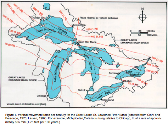
Map showing differential recent uplift associted with the last ice age. As would be expected, the area towards the ice mass center which was depressed more, is rebounding at a greater rate. What might be the implications for shoreline processes along the lake shore? Image from NOOA report, 1999, Proceedings of the Great Lakes Paleo-Levels Workshop: The Last 4000 Years; Cynthia E. Sellinger and Frank H. Quinn, Editors (accessed 11/7/17).

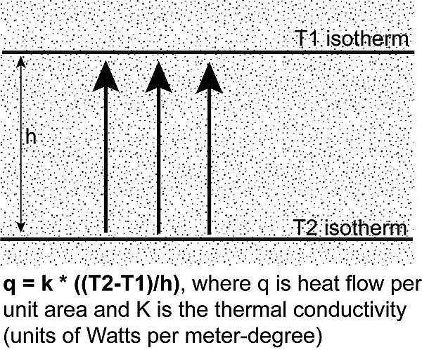
As the oceanic or any type of floating crust cools its density changes, and thus it will float at a different level. It cools because it starts out as recently crystallized igneous material, and then the heat flows out of it with time. Thus, the profile of the oceanic spreading ridges (with all the bumps and warts taken out) could be thought to reflect a simple history of conductive cooling with time. In words, the basic equation for equilibrium heat flow is that the heat flow is equal to the temperature difference in the direction of heat flow at two points aligned in the direction of heat flow times the thermal conductivity all divided by the distance between the two points.

Combining equations for isostasy and for heat flow for a spreading ridge allows one to model the large scale topogrpahy of the ocean ridge. An equation, taken from Turcotte & Schubert (1982), that describes this model is as follows:

Y depth = [( 2 * pm * am * (Tm-To))/ (pm-pw)]* {(km * x )/(pi * uo)}^.5

This can be shortened to:

Y depth = k * {(km * x )/(pi * uo)}^.5 where k = [( 2 * pm * am * (Tm-To))/ (pm-pw)]

Where:

Y depth = depth below the ridge crest elevation.
pm = mantle density, average value of 3250 kg m^(-3)
pw = water density, average value of 1000 kg m^(-3)
am = coefficient of thermal expansion for mantle rocks. Typical value = 3*10^(-5) degrees K^(-1)
Tm = temperature at base of lithosphere in Kelvin (constant T with time) = 1250 degrees Celsius.
To = temperature at top free surface heat is radiating out at in Kelvin. This is pretty close to 0 degrees Celsius for the bottom ocean waters.
km = thermal diffusivity of mantle rocks. Typically 1 mm^2 s^(-1)
x = distance away from ridge center
uo = spreading rate.

Note that x /uo gives the age of the crust. Actual and modeled topographic profiles for specific ridges show a decent fit (better than 85%), with some consistent differences between the model and the observed. The ridge crest areas are not quite as high as the model would predict, and the extreme flanks are higher than the model would predict. Note, also that when thinking about units you will need to have common units for distance and for time in particular for this equation to work. Perhaps change all the distance units to meters, and time units to seconds when using this equation in your exercise.

Afternote: While not within the scope of this course to pursue in detail, it is interesting to note that this equation does a very good job of describing seafloor topography, there are some consistent departures of reality from the model. For example, the area around the spreading ridge is consistently lower than the equation would predict. Can you think of why? An additional consideration is the phenomena of non-unique solutions in geophysics. Could a different physical model produce the same results? While this is a permissible model given constraints, sometimes there are other permissible models that could also explain the reality.

The following is mainly taken from Turcotte & Schubert (1982) which provides derivations. It is a modification of the model for cooling continental lithosphere and basin formation. If lithospheric thickening and cooling (a half-space cooling model) is responsible for the subsidence (and a bunch of other assumptions are acceptable) then this equation may work.

Y subsidence = [( 2 * pm * am * (Tm-To))/ (pm-ps)]* (km * t / pi)^.5

The values are as above in the case for the cooling spreading ridge. The one difference being the ps = density of sedimentary rock (typically 2500 kg m^(-3)).

Check units when using this equation. Note that basically this boils down to Y subsidence is a square root function of time. Note that are a whole slew of assumptions behind this that could be violated in any particular case (see Turcotte & Schubert for particulars). For what type or phase of basin might this work? Perhaps the post-rift faulting phase of an extensional basin.

How can you test how well this model describes basin subsidence? Plot the cumulative basin thickness versus time and see if it follows the appropriate line. There is a nice example in Turcotte & Schubert (1982).

The rate can be described by the equations below:

C = Co * e ^ -(k*t)

ln C = ln Co ­ (k*t)

where Co concentration at the start of a reaction, C concentration at time t during the reaction, k is the rate constant.

If you want to find k experimentally you can measure concentrations with time and then graphically solve for k. Rates of metamorphic or hydrothermal reactions could be investigated in such a framework. Again, think about equilibrium issues.

Here are some other examples:

• Allometric growth in organisms: The basic idea is that the "relationship between the size of one part of an organism and the size of another is not linear but follows the general equation y = B * x^a." (Ferguson, 1988). This is apparent for children. This would be a power law function.
• Crater/impact flux rate with time: exponential decay?
• Stream profiles and hydraulic phenomena (Mayer, 1990):
• Tertiary or accelerating creep.
• Stream branch development with time.
• Sediment compaction, dewatering and density changes.

This non-linear behavior shows up quite a bit in the real world!!

References:

• Ferguson, J., 1988, Mathematics in Geology, Allen & Unwin, London, 299 p.
• Mattox, S. R., 1999, An Exercise in Forecasting the Next Mauna Loa Eruption: Journal of Geoscience Education, v. 47, p. 255-260. Describes use of exponential probability equation in the context of predicting volcanic eruptions.
• Mayer, L., 1990, Introduction to Quantitative Geomorphology, Prentice Hall, 380 p.
• Sharma, P. V., 1986, Geophysical Methods in Geology, Elsevier, 442 p.
• Shea, J. H., 2001, Teaching the mathematics of radiometric dating: Journal of Geosciences Education, v. 49, p. 22-24.
• Turcotte, D. & Schubert, G., 1982, Geodynamics, Wiley, 450 p.
• Vacher, H. L., Computational Geology 9 ­ The Exponential Function; Journal of Geoscience Education, v. 48, p. 76.

Copyright by Harmon D. Maher Jr.. This material may be used for non-profit educational purposes if proper attribution is given. Otherwise please contact Harmon D. Maher Jr.