 Lab 2: Structure contour mapping (20
pts.):
Lab 2: Structure contour mapping (20
pts.):Lab 2: Structure contour mapping (20
pts.):
Lab goals:
Example of a structure contour map from the USGS. The strcture is basically that of an asymmetric syncline with a steeper SW limb. Image source: https://pubs.usgs.gov/dds/dds-033/USGS_3D/ssx_txt/geology.htm .
Structure contour maps are basically the same as topographic maps, where the surface being mapped is some geologic surface, often in the subsurface. Geologic surfaces commonly mapped in this way are:
However, one can get much more sophisticated and contour for example the amount of offset on a fault surface (which shows a very interesting pattern). As we will see in later labs one can also map the density of point data.
There are some differences between standard topographic maps and structural contour maps. Your surface does not have to be continuous everywhere, but can be truncated. For example the surface created by the top of a sill can be truncated by a fault.
You can also contour and 'map' other features than a physical surface. In this case the z axis instead of being elevation can be any physical/chemical parameter. For example, you can contour geophysical parameters such as the acceleration of gravity, or the strength of a magnetic field. When working with contaminant plumes the z parameter is the concentration of some contaminant. Isopach maps are where you are contouring the thickness of some unit.
When contouring you are assuming that for some area with data located by x, y values, the z values form a smooth continous surface.
Trig functions for a right triangle:
Exercise 1: structure contours. Use one of the three structure contour maps provided below (as specified by the instructor) to answer the following questions. The assumption here is that there is no significant topography.
a) The contours shown are on a fault surface and the numbers are meters above sea level. What is the strike of the fault (you will need a protractor to answer this)?
b) What direction does the fault dip in?
c) What is the dip angle? You will need to measure the perpendicular spacing between the strike lines and then use the appropriate trig function above to compute the dip amount. Remember to measure the distance between the strike lines in a direction perpendicular to the strike lines.
d) The center of the star marks a point on the top of a stratigraphic formation that is truncated by the fault. In the top map the planar surface is oriented N20E - 40SE (orientations for the other two are given on the map). Draw and label a strike line for the top surface of a stratigraphic formation so that the strike line truncates against the equivalent structure contour for the fault.
e) Compute the map distance between strike lines for the stratigraphic formation top with a 100 m contour interval using the appropriate trig function. Report that distance here.
f) Draw the structure contours for the stratigraphic formation top that match the fault structure contour values, truncating each of them against the equivalent fault structure contour. You will need to use your map scale to convert the real distance to the map distance.
g) Draw and label the cut-off line, which is the line formed by the truncation of the stratigraphic formation top surface against the fault surface.
h) Use the protractor to measure the trend, the angle from N of the cut-off line, using the quadrant the line descends towards.
Bonus (1 point): Draw the structure contours on the other side of the fault if there was 150 m of dextral offset.


Relationships between structure contours for a planar surface, a topographic surface and the map expression on the map of the planar surface.
You saw in the above exercise how one can map the line created by the intersection of two surfaces. You basically connect the points created by the intersection of the contours of equal elevation of the two respective surfaces to create what the map pattern should be. You of course can do the opposite, connect the points where the line representing the map expression crosses the same contour to estimate the structure contour line at the elevation of the contour.
Exercise 2: Geologic contacts, structure contours and topographic contours. There are two options below. Complete the assigned one.
Option1: Use the map diagram below to complete the following. The thicker dotted line represents topographic contour lines, the thinner continuous line represent contours on a fault surface, and the red (grey in b&w) represents the topographic surface/map expression/trace of the fault surface.
a) A second fault surface exists exactly 100 meters elevation below the one depicted below. Draw its map expression (the equivalent of the red line for the second fault).
b) A horizontal bed is cut by these faults. In the footwall of the lowest fault it is at an elevation of 350 m. In the footwall of the higher fault it is at an elevation of 290 m, and in the hanging wall of the higher fault it is at 210 m elevation. Draw in the map expression of the horizontal bed as it is cut by these two faults. You will need to interpolate between the given contour lines. Remember that the footwall is the block beneath a dipping fault, and the hanging wall is that above.
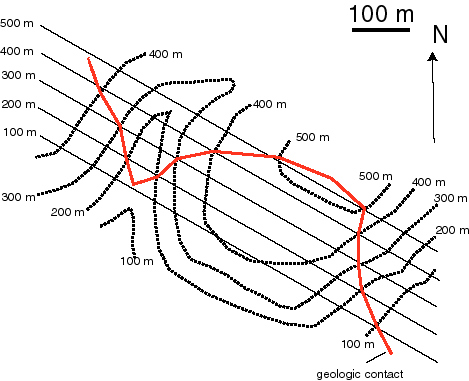
Map for option 1.
Option 2: In the image below the red lines are structure contours on a fault, and the black lines are topographic contours.
a) Trace out the map expression (the implied trace of the fault at the topographic surface given the information provided). Finidng points where topogrpahic and structure contours of the same value cross is the key. Is the fault dipping above or below 45 degrees?
b) There is an additional upper fault, 100 m directly/vertically above the fault you have drawn. Draw its map expression (hint: the 500 m contour on the lower fault would be the 600 m structure contour on the upper fault).
c) The same horizontal stratigraphic horizon is at 290 m elevation in the footwall of the lower fault, and at 310 m elevation in the hanging wall of the lower fault, and is at 410 m elevation in the hanging wall of the upper fault. Draw in their map expression using a different color (and label what is fault versus stratigraphic horizon on your diagram). You will need to interpolate between the given topographic contours and their elevations.
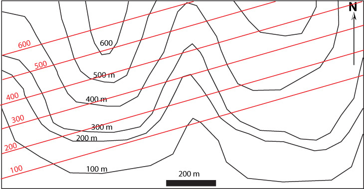
Map for option 2.
Hand contouring point x,y,z data.
While computer programs conduct this type of analysis readily, it is useful to hand contour data also. In some cases it can be argued that an experienced geologist might produce a better contour map of a surface than the computer does because they can use their expert knowledge of how that type of geologic surface behaves.
When contouring you will first need to chose a contour interval. You want the smallest contour interval possible without overinterpreting the data (producing false accuracy). A general rule of thumb is that if you commonly have several contours passing between two control/data points then your interval is too small. One approach is to find the range (the highest minus the lowest value) and divide by the number of data points you have. Your contour interval should be larger than this value. Too large of a contour interval will lead to an oversimplified interpretation. Conventionally, contour values are also values rounded up near to the place value of the contour interval - in other words if your contour interval is 100 units, you wouldn't have a line at 225, 325, 425 .... . Instead you would do 200, 300, 400... .
Use your geologic knowledge to guide your contour construction.
Favor the simplest interpretation that the data permits (in this case the simplest surface possible). Don't over interpret so that surface features are indicated which could exist, but that the data doesn't constrain to exist.
The contour map product is an interpretation since interpolation and significant discretion of exactly where you draw the lines can exist. What are some rules of interpolation between two constraining control points? A simple approach is to position the contour proportionally. If the control points are at 60 and 30 units, then the 50 unit contour interval should be 2/3rds the way along a line as your travel from the 30 to the 60 point. Other better rules of extrapolation exist.
Where should you start contouring? Where you start can make a difference, since one tends to use the initial contours drawn as a guide to help you draw the subsequent contours under construction. One suggestion is to start where the surface is best constrained, where you have the maximum density of points, and then to work to areas where the surface is less constrained. This usually means starting in the middle of the map and in the middle range of the contour elevations being constructed.
Exercise 3 - hand contouring: There are 2 options below. Please do the one assigned.
Option 1: Below
is a map of drill hole data, showing the elevation in feet above
sea level of the Tarkio limestone. This is in the area of the
Humboldt fault zone, SE Nebraska. Hand contour the data, also interpreting
where you think the faults may lie. There will be a lot of interpretation/discretion
involved in how this map looks. Make sure your contours and any
faults are well labeled

Option 2: The data points are elevation in meters above sea level of a stratigraphic contact in an area close to Buffalo, Wyoming. After contouring by hand, describe what type of structural feature exists and what the orientations of various parts of the feature are.

Computer contouring:
Computer contouring and visualization of the surfaces created is a marvelous tool. However, don't let it be a black box, magical sort of endeavor. You should understand at some level how the computer is generating that surface. There are different ways and the results can be quite different. For those of you who took geodata you can review, or for those of you who want to learn more about how the computer contours data, you can read material at the relevant geodata lecture notes.
Exercise 4: Using Surfer
Option 1: Below is x,y, z data in feet for the option 1 area you hand contoured above.
a) Enter the data into a software package that will contour the data and produce a contour map. If you are using Surface 3 on a Mac, then save this as comma delimited text. Surfer can open it up as an Excel sheet.
b) Compare the computer generated map with your hand contoured map. What is the difference?
c) Generate a 3-D diagram that shows the surface from a instructive vantage point.
d) Describe what can you conclude about any fault in this area?
| 1884.056 | 16237.98792 | 1080 |
| 3104.712 | 15707.33472 | 1075 |
| 2573.992 | 14115.37512 | 1090 |
| 6819.752 | 19687.23372 | 1003 |
| 5492.952 | 18015.67614 | 1054 |
| 8040.408 | 18201.40476 | 1010 |
| 5201.056 | 16874.77176 | 1070 |
| 7881.192 | 17272.76166 | 1019 |
| 9552.96 | 17352.35964 | 904 |
| 8305.768 | 16609.44516 | 1036 |
| 5572.56 | 16237.98792 | 1074 |
| 5890.992 | 15070.55088 | 1078 |
| 13002.64 | 20085.22362 | 681 |
| 12684.208 | 18387.13338 | 656 |
| 11914.664 | 17272.76166 | 672 |
| 10985.904 | 16848.2391 | 598 |
| 15656.24 | 17511.5556 | 665 |
| 12896.496 | 15442.00812 | 694 |
| 10959.368 | 14672.56098 | 738 |
| 10879.76 | 13664.3199 | 902 |
| 11543.16 | 13160.19936 | 788 |
| 14037.544 | 13266.33 | 703 |
| 12949.568 | 12205.0236 | 693 |
| 15470.488 | 12337.6869 | 705 |
| 17460.688 | 18201.40476 | 655 |
| 16929.968 | 15839.99802 | 659 |
| 16001.208 | 14619.49566 | 689 |
| 18071.016 | 14486.83236 | 666 |
| 16956.504 | 12682.61148 | 708 |
| 11967.736 | 8941.50642 | 690 |
| 10879.76 | 7747.53672 | 700 |
| 10614.4 | 7137.28554 | 763 |
| 10295.968 | 11753.96838 | 910 |
| 7668.904 | 11833.56636 | 1060 |
| 5201.056 | 11860.09902 | 1108 |
| 4670.336 | 6341.30574 | 1108 |
| 7695.44 | 6447.43638 | 1080 |
| 5147.984 | 1406.23098 | 1070 |
| 9367.208 | 2573.66802 | 1072 |
| 10534.792 | 5810.65254 | 891 |
| 10694.008 | 3714.5724 | 1002 |
| 13108.784 | 1645.02492 | 977 |
| 12233.096 | 769.44714 | 997 |
| 11967.736 | 557.18586 | 1002 |
| 15284.736 | 928.6431 | 925 |
| 15815.456 | 2149.14546 | 907 |
| 14939.768 | 4643.2155 | 720 |
| 14886.696 | 5810.65254 | 703 |
| 17726.048 | 6367.8384 | 683 |
Option 2: Below is x,y, z data in meters for the option 1 area you hand contoured above. The X and Y values are UTM.
| UTM Easting (m) | UTM Northing (m) | strata elevation |
| 726895 | 4943927 | 1353 |
| 726978 | 4944084 | 1376 |
| 726748 | 4943787 | 1303 |
| 726801 | 4943501 | 1254 |
| 726794 | 4943400 | 1232 |
| 726772 | 4943185 | 1194 |
| 726871 | 4942934 | 1149 |
| 727369 | 4944148 | 1222 |
| 727499 | 4944131 | 1144 |
| 726882 | 4944308 | 1393 |
| 727056 | 4944396 | 1296 |
| 726994 | 4944518 | 1242 |
| 726802 | 4944594 | 1338 |
| 726750 | 4944451 | 1395 |
| 726617 | 4944793 | 1283 |
| 726695 | 4944673 | 1335 |
| 726487 | 4944685 | 1410 |
| 726379 | 4944917 | 1367 |
| 726288 | 4944845 | 1432 |
| 727759 | 4943870 | 1193 |
| 727825 | 4943641 | 1304 |
| 727495 | 4943751 | 1357 |
| 727162 | 4943373 | 1294 |
| 727504 | 4943302 | 1346 |
| 727235 | 4943110 | 1266 |
| 727107 | 4943092 | 1237 |
| 727072 | 4942917 | 1194 |
| 727017 | 4942761 | 1140 |
| 726267 | 4944054 | 1286 |
Link to associated Excel File.